What is Delftia?¶

delftia%20cluster%20and%20protein.png Delftia is a genus of bacteria with a bunch of cool features! The best studied species, Delftia acidovorans can produce gold nanoparticles from gold ions in solution. This bacteria has been found living in biofolms with Cupriavidis metallidurans on gold nuggets(1). It is also found in soil, in sinks and in rhizospheres of different plants where it promotes their growth(3).

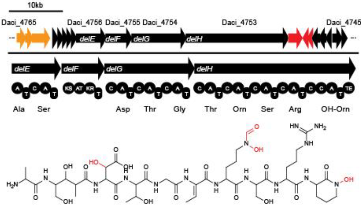
Delftia acidovorans forms gold nuggets by producing a short nonribosomal peptide called delftibactin (1). The 16 genes responsible for the production of delftibactin are called the del cluster (delA-delP) (1). These genes were originally discovered in Delftia acidovorans SPH-1, but our research shows that the del cluster appears to be present across the genus (1).

http://2013.igem.org/Team:Heidelberg/Project/Delftibactin

The Phylogenetic Classification of Delftia¶

Proteobacteria

Betaproteobacteria

Burkholderiales

Comamonadaceae

Delftia

How will we find Delftia?¶

Our Workflow:

Narrative%20Methods%20Figure.png

Each step will be outlined before you reach it with a description of the apps, parameters and results.

We'll start with a number of raw reads, clean them up and do a little taxonomy to figure out what we might be able to assemble. Next, we'll assemble the reads using 4 different methods and pick out the best assembly. Then we'll take those reads and sort them by genome and assess the quality of those genomes. We'll select the high quality genomes to annotate and insert into phylogenetic trees to find relatives.

Learning Objectives:¶

After completing this narrative, students will be able to:

Describe the steps of assembling metagenomic data into genomes and the importance of each step.
Define the following terms and processes, read trimming, contig(s), bin(s), binning, MAG, L50, and N50.
Interpret the results of FastQC and CheckM reports.
Explain why multiple assemblers are used.
Compare and contrast assembly statistics to determine the best assembly to generate MAGs.
Identify high quality bins to extract and annotate.

What samples am I searching for Delftia?¶

Sample 1: Metagenome generated from fracture fluid collected July 12-27, 2012 from a borehole located on the 26 level of Beatrix Gold Mine (Welkom, South Africa) 1,339 m below land surface.

Bio Sample: SAMN04419121; Sample name: Be326_2012_DNA_MF; SRA: SRS1792548 Link to more information: https://www.ncbi.nlm.nih.gov/biosample/SAMN04419121

Why did I pick this sample?

Delftia acidovorans and Cupriavidus metallidurans make up 90% of the bacteria found in biofilms on gold nuggets (1). This sample is from a gold mine, so it would be interesting to see if Delftia is also present here. Additionally, the Krona plot indicated that there were some (unassembled) sequences that resembled Delftia.

Sample 2: Hydraulically fractured gas well metagenomes fluid from sample at timepoint_82

Bio Sample: SAMN04417545; Sample name: Timepoint_82; SRA: SRS1256393 Link to more information: https://www.ncbi.nlm.nih.gov/biosample/SAMN04417545

Why did I pick this sample?

Delftia is often found in soil and water. It is capable of using a diverse array of carbon sources as well. (That's why so many studies focus on it's use for bioremediation.) In this case the Krona plot indicated a small portion of potential Delftia sequences.

Sample 3: Subsurface sediment microbial communities from gas well in Oklahoma, United States - OK STACK MC-FT3-sol metagenome

Bio Sample: SAMN09199659; SRA: SRS3667068; DOE Joint Genome Institute: Gp0290895 Link to more information: https://www.ncbi.nlm.nih.gov/biosample/SAMN09199659

Why did I pick this sample?

I stumbled upon this sample while I was searching through the database. The Krona plot showed a much greater proportion of genes that could potentially be from Delftia, and I couldn't skip it. Delftia is often found in soil and/or sediment.

Sample 4: Metagenome of iron plaque on rice root from As contaminated paddy soil, sample from Yanhong

Bio Sample: SAMN07211852; Sample name: YanhongMeta01; SRA: SRS2392319 Link to more information: https://www.ncbi.nlm.nih.gov/biosample/SAMN07211852

Why did I pick this sample?

I choose this sample because it brings together soil and aquatic environments that Delftia can be found in and is associated with heavy metals. The Krona plot indicated some Delftia-associated sequences are present from several species of Delftia.

Sample 5: Peat soil microbial communities from Stordalen Mire, Sweden - IR.F.S.T-25

Bio Sample: SAMN09201211; SRA: SRS3568559,DOE Joint Genome Institute: Gp0256443, Link to more information: https://www.ncbi.nlm.nih.gov/sra/SRX4415252[accn]

Why did I pick this sample?

I picked this sample because soil is one of the common sources of Delftia. The Krona plot looked promising as well for both Delftia acidovorans and Delftia tsuruhatensis.

Step 1. Import Metagenomic Data¶

The data I'm using comes from publicly available datasets available from NCBI's Sequence Read Archive (SRA).

The sample you need to upload should be a metagenomic sample listed as a WGS having paired reads. Your sample cannot be more than 20G bases or you'll need to import it through Globus (see this link for more information). You can also check out this really informative narrative for an in depth view of how to upload data from other sources: https://narrative.kbase.us/narrative/48493

App: Import SRA File as Reads from Web

Timing: 1-5 hours depending on the size of the file and queue time. (Its often helpful to run this in the morning so it uploads and then you can set up the assembly to run overnight or over the weekend.)

View Configure:

SRA URL: Use the first link from the "Reads Access" page and paste it into this block.

Reads Object Name: this will be what your sample is called once it's been uploaded into KBase. Make sure its something you'll be able to remember and follow the workflow with.

Sequencing Technology: Select the sequencing technology that was used to call the reads.

Single Genome: These reads are all metagenomes, so you don't need to select this box.

Results: Your reads should appear in the Data panel to the left. Before proceding, double check that they are a PairedEndLibrary. If they are a SingleEndLibrary, you'll need to select a different sample, because your assembly won't work with a SingleEndLibrary. In the results panel itself you'll see some stats from the reads including the number of reads, quality score mean and mean read length.

Step 2. Assess the Quality of your Samples¶

You've uploaded your data, great! Now you have to check the quality of the reads. First assess quality with FastQC. Then, if you need to, trim the reads and assess quality again to make sure the low quality reads have been removed from the sample.

Apps:

Timing: 5-20 minutes depending on queue and the number of reads

Assess Read Quality with FastQC View Configure:

All you need to imput to assess quality is the name of your reads library

Results: This app will give you a full report of the quality of your reads. The report will have two pages, for the forward and reverse reads in the PairedEndLibrary. Here we'll be focusing on the Per Base Sequence Quality, but the rest of the report offers a bunch of useful information about our library.

Per Base Sequence Quality: An overview of the quality scores for each position in the read. The red line is the median, blue the mean, the yellow bars the interquartile range and the black lines the 10% and 90% points.
Per Sequence Quality Scores: This shows the distribution of quality scores across sequences. Ideally you will only see a single peak on the far right. If you see a second peak to the center or left, you may have a subset of low quality reads that need to be trimmed out.
Per Base Sequence Content: This shows the proportion of each base present at each position in your reads. In a perfectly random run, you would expect to see parallel lines across this chart, but the relative amount of each base would depend on the genome(s) sequenced.
Per Sequence GC Content: In a random library, you would expect this to fall across a normal distribution with a peak over the GC content of the chromosome. An unusually shaped distribution can indicate contamination or systemic error.
Per Base N Content: Whenever a base is unable to be called, the sequencer labels it as N for any nucleotide. This chart shows the percent of bases at each postition that have been called as "N". It's not unusual to see some of these at the end of sequences when the quality drops, but a consistently high proportion or a peak in the start or middle of the sequence may indicate a problem in the analysis.
Sequence Length Distribution: This shows the distribution of read sizes.
Sequence Duplication Levels: This plot shows the relative number of sequences with each degree of duplication. It's based only on a subset of the data, but you should get a good idea of how many sequences have duplicates. If there are a number in the 2 or more, you may need to trim the library to remove them.
Overrepresented Sequences: If any sequences represent more than 0.1% of the total sequences, they will be listed here. An abundance of any sequence may indicate contamination, a lack of diversity in the library or is biologically significant.
Adapter Content: This graph shows where any adapters are found in your library.
Kmer Content: If any Kmers are overrepresented in your library, they will be listed here.

For a more in depth look at understanding your FastQC report, check out the manual here: https://dnacore.missouri.edu/PDF/FastQC_Manual.pdf

Trim Reads with Trimmommatic View Configure

Read library or set: Select the library you want to trim.
Parameters: This section covers different trimming parameters specific to removing adapters, croping the sequences, and the quality thresholds required to trim a read. In this workflow, I'm going to leave them all as defaults, but you can learn more about them in the App Info page and in the KBase App catalog.
Output library name: Make sure to specify that this library has been trimmed so you can tell the two libraries apart later.

Once you've trimmed the read library, reassess the quality of the PairedEndLibrary using FastQC.

Results: A FastQC Report that details the quality of the reads you've submitted and possibly trimmed libraries.

Q1 Looking at the results of the FastQC app, which reads set(s) would you choose to trim and re-assess the quality of? Why did you pick that/those set(s)?

Step 3. Taxonomy Before Assembly¶

Before we assemble these libraries, it will be helpful to get an idea of what's present in our samples and at what abundance. KBase has two apps to do this, Kaiju and GOTTCHA2.

Apps:

Timing: 20 mins-2 hours depending on queue and number of reads you're running

1. Classify Taxonomy of Metagenomic Reads with Kaiju

This app translates reads into proteins and uses those sequences to identify what's present or possibly present in the sample.

View Configure:

Read Library or Set: You can either run the app for each library or run it once with all read libraries.
Taxonomic Level: By default the app will show all levels from phylum to species.
Reference DB: Here you'll select the database to compare your reads against. Either RefSeq or BLAST are fine for our purposes and you don't need to include eukaryotes, since we're just looking for a bacteria.
Low Abundance Filter: This value filters out taxa that occur infrequently in your sample and helps simplify your results. After all, if something is present in low abundance, you're unlikely to be able to produce an assembled genome from a small amount of reads. The default is fine, but if you want to look at what is present in low abundance you can lower it.
Subsample Percent, Subsample Replicates, and Subsample Seed: To save time Kaiju only looks at a subsample of your reads. These settings allow you to adjust the percentage of your sample and replicates that Kaiju uses. In a truly random sample, there should be no variation between them, and this is generally true and can be seen below in the individual runs.
Filter Low Complexity: This should be set to filter so the algorithm only takes unique protein sequences into account.
Allow Imperfect Matches? Min Match Length, Allow Imperfect Matches, Greedy Max Mismatches, Greedy Min Bit Score, Greedy Max E-Value: These settings all relate to how much you want the algorithm to tolerate mismatches in protein sequences. How specific you want it to be is up to you, in this case we don't need it to be extremely specific since we only want a quick overview of what's present.
Sort Plots By: How you sort the plots is up to you, mine are sorted by total abundance, but you can also sort them alphabetically.

Results: Your results will be a series of tables showing the breakdown of your sample beginning with the phyla and ending at species. The tail includes everything that is present below the low abundance filter.

2. Classify Taxonomy of Metagenomic Reads with GOTTCHA2

Unlike Kaiju, this app shows relative abundance based on unique nucleotide sequences from RefSeq.

View Configure:

Read Library/Set: Add your reads library here.
Reference DB: You can either select the bacterial/viral/archaeal database or fungal database. In this case, we'll be using the first option.
Minimum Coverage: This is the minimum percentage of the unique genome signatures identified to be considered in the abundance calculation. Decreasing it will include lower abundance species, while increasing it will remove them.
Minimum Reads: The minimum number of reads to be included in the abundance calculation.
Minimum Length: The minimum length of reads for them to be included in the abundance calculation. If your library contains many short reads, you may want to reduce this value, but be aware that reducing it also increases the chance that you will get an incorrect result.
Maximum Zscore: This is based on the estimated Zscore. The default is fine for our Delftia search.

Results: There are three ways you can view the results from GOTTCHA2. The first is as a table showing the classification of your reads, some statistics regarding their abundance and their relative abundance. The second is as a phylogenetic tree showing the relationships of the different taxa identified in your sample. The third layout is as a Krona plot, an interactive plot that displays relative abundance and phylogenetic relationships. Clicking on a phylum will zoom in to show the classes within it. How far you can zoom down depends on the sample and the unique sequences in it.

These first two runs of Kaiju include the first 4 libraries run as one first with NCBI BLAST as the database, then with RefSeq as the database. The following 4 examples show the libraries individually with different settings to increase the proportion of the library represented.

These runs of Kaiju are broken down by sample and use the NCBI BLAST database. They are run on two subsamples.

Q2 Do the two subsamples vary much? Is this expected or unexpected and why?

This first run of GOTTCHA2 includes ALL read libraries as one sample. The 4 runs afterwards show the samples individually.

Q3: Open the Krona plot from this sample. Viruses make up what percent of the sample?

Q4: What is the relative abundance of Betaproteobacteria in this sample?

Q5: Which sample(s) look the most promising based on the taxonomy results from GOTTCHA2?

Step 4. Assembly of Metagenomic Data¶

Alright, you've made it this far. This step takes the longest, so you may want to set it up to run overnight or over the weekend. This step will take our read libraries and line them up into longer sequences called contigs. Later we'll sort these contigs based on what genomes they came from. We'll be using three different apps to generate 4 different sets of contigs.

Apps:

Timing: hours to days (One of my assemblies below ran for almsot 4 days.)

1. Assemble Reads with MetaSPAdes

View Configure:

Read Library: Add your reads here. If you trimmed your library, be sure to use the trimmed version. MetaSPAdes will ONLY accept a PairedEnd Library.
Minimum Contig Length: The smallest contig the assembler can produce. Larger contigs have a higher chance of containing a whole gene or unique sequence, but there will be fewer of them. Smaller contigs have a lower chance of containing a whole gene and can wind up contaminating your genomes if they are binned incorrectly. However, there will be a lot more of them. The default here is 2,000 and that's what I'm sticking with below for all my assemblies.
K-mer Sizes: K-mers are used in the assembly process to look at the contigs to look for overlapping regions. If you want to learn more about this process, check out this video.
Assembly Only(no error correction): Don't select this, for our search we want to correct for any errors that may occur.

2. Assemble Reads with MEGAHIT (run 2x)

View Configure:

Read Library: Add your reads here. If you have trimmed the library, use the trimmed version. MEGAHIT will only accept a PairedEnd Library.
Parameter Preset: You'll run this app twice, once set at "Meta-sensitive" and again set at "Meta-large."
Minimum Contig Length: The default here is fine, 2,000 bp is a good size for your smallest contig, at that size hopefully they'll all contain some identifying feature(s).
K-mers: I left these at their defaults. If you want to learn more about K-mers and their role in assembly, check out the video above.
Output Assembly Name: Be sure to specify in the name which parameter preset you used to create the assembly.

3. Assemble Reads with IDBA-UD

View Configure:

Reads Library: Add in your reads here. If they have been trimmed, you should add in the trimmed, paired library. IDBA-UD can accept a SingleEnd Library, but you should use the PairedEnd library.
Minimum Contig Length: This sets the size for the smallest your contigs can be. The default is 2,000.

Results: Regardless of the assembly you use, you'll get the same result; a QUAST report. This report details the major features of your assembly and important statistics, such as the length of the longest read, the number of reads longer than 1,000,000 bases, the N50 and L50. In the next step we'll compare these statistics and receive a visual representation of the key parts of this report. For now, take note of which assembly contains the most base pairs.

Sample 1. "Subsurface Gold Mine Reads"¶

Sample 2. "Hydraulic fracture well fluid"¶

Sample 3. "Subsurface gas well"¶

Q6 How long did it take (including the queue time) to assemble this reads dataset with metaSPAdes?

Sample 4. "Rice Root Iron Plaque Reads"¶

Sample 5. "Peat Soil"¶

Step 5. Compare assemblies¶

Success! You've created 4 different assemblies from your metagenomic data. Now, you need to pick the best to sort out all those contigs into genomes. That step, sorting the contigs into different genome bins is called binning. Each bin will represent a single genome, but more on that later.

App: Compare Assembled Contig Distributions

Timing: 5-10 mins.

View Configure:

All you need to add here are your different assemblies from above. For example, in the first run I'll compare the Subsurface_gold_mine_meta_sensitive_MEGAHIT.assembly, subsurface_gold_mine_meta_large_MEGAHIT.assembly, subsurface_gold_mine_IDBA.contigs, and subsurface_gold_mine_SPAdes to determine which is the best to use moving forward.

The Results: A report showing the different statistics from each assembly. Some key features of this report include:

N50: the contig length such that using longer or equal length contigs produces half the bases of assembly.
L50: the minimum number of contigs that produce half of the assembly.
The length of the longest contig.
Histograms showing the distribution of contig lengths.

A good assembly will have:

A longer largest contig.
More contigs over 100,00 bp long
More contigs over 1,000,000 bp long.
A high N50.
A low L50.

A bad assembly will have:

A short longest contig.
Few contigs over 100,000 bp long.
No contigs over 1,000,00 bp long.
A low N50.
A high L50

Q7a Which assembly would you use for binning contigs from this sample? Why did you pick that assembly?

Q7b Which is the worst choice for binning contigs? Why is it the worst?

Q8 Which assembly should I use to bin the contigs from the hydraulic fracture well fluid sample? Why?

Q9a Which assembly is the best for binning the contigs from the subsurface gas well sample? Is there more than one option? If so, which one would you use and why?

Q9b Which assembly can you rule out?

Q10 Which assembly should I use to bin the contigs from the rice root iron plaque sample? Why?

Q11 Which assembly should I use to bin the contigs from the peat soil sample? Why?

Step 6. Bin your Contigs¶

Alright, you've picked the best assembly, now you'll sort all the contigs into bins that each represent a single genome. This step is called binning the contigs.

App: Bin Contigs using MaxBin2

Timing: 2+ hours depending on the number of contigs and bins present in your sample.

View Configure:

Assembly Object: Put your best assembly here.

Read Library: This is the library the contigs were generated from. If you needed to trim your read library, use the trimmed reads.

Probability Threshold: The confidence the alrogrithm must have for a contig to be placed within a bin. If a contig falls below this cutoff, then it will be left as unclassified. The default is 0.8.

Marker Set: MaxBin2 can bin both bacterial and archaeal genomes. In this case we're only looking at bacteria, so keep it set to the bacterial marker gene set.

Minimum contig length: Any contigs shorter than this will be ignored when binning. 1000 is the default, but above we set our contig minimum length at 2000 so we can increase this to 2000 or leave it as is, since we shouldn't have any contigs shorter than 2000 bases.

Results: The output from this app opens in a new section. The first panel lists the number of bins (and maximum number of genomes) and nucleotides included in all the contigs. The second tab offers some detail about the different bins including marker completenes, GC content, the number of contigs in each bin and their total length. To see information about the individual contigs in a bin, click the bulleted list icon for that bin or the graph beside it. However, these results tell you nothing about the quality of the bins, they could be highly contaminated or contain multiple copies of the same set of genes.

Q12 Delftia acidovorans has a GC content of 66.7%. Based on GC content alone, do any of these bins match D. acidovorans?

Q13 What is unusual about the bins from the hydraulic fracture well fluid sample?

Hint: look at the bins tab.

Step 7. Check Bin Quality¶

You should now have a bunch of different bins. Each bin represents a single genome (in theory). In this step we'll check these bins for their completeness, contamination and any duplicates using CheckM.

App: Assess Genome Quality with CheckM

Timing: Depends on the number of bins in your sample and the reference tree you pick

View Configure

Input Assembly, Genome or BinnedContigs: Add in your set of bins from the last step here.

Reference Tree: You can either select the full tree or reduced tree to compare your bins to. The full tree takes longer, but is recommended for a better understanding of what each bin represents. However, if you're tight on time the reduced tree is fine since we'll be generating a species tree to determine close relatives of our assemblies later.

Save all Plots: Save will allow you to download a .zip file of the resulting genome quality plots. Don't save will not.

Results: CheckM will give you two forms of the same report, a graphic version and a table. I think the table is easier to understand, so that's what I'll be covering here. The first column shows the bin name. They're all just numbered bins at this point, but you can rename them later if you want. The second column shows the lineage of the markers present in that bin. Some will be more specific than others, depending on the bin, its completeness and contamination. Number of genomes is the number of genomes used to create the marker set, and number of markers is the number of markers generated. These markers are unique and are expected to occur only once in the genome, replicates indicate contamination. The columns 0 through 5+ indicate the additional copies of these marker genes and are used to calculate contamination. Be aware that contamination is an underestimate in this app.

The last two columns indicate the completeness and contamination of your genome as percents. High quality genomes are over 90% complete with less than 5% contamination. However, since we're just looking to ID if Delftia is present, I'm using any genomes over 75% complete with less than 5% contamination. If an assembly falls outside this range, but looks promising, you can keep it, but be sure to note that it's a low quality assembly.

Write out a list of all the bins you want to keep, it will be useful in the next step.

Q14a Which bins would you select to keep working with?

Q14b Why did you pick those bins?

Q15 Are any of these bins high enough quality to keep working with? If so, which one(s)?

Q16 This one looks more promising! Which bins would you choose to extract and are there any that look like Delftia?

Step 8. Extract Assemblies¶

Up above you checked the quality of all your bins and picked out all the ones that were over 75% complete and less than 5% contaminated. Now you're going to separate them from the contaminated and incomplete assemblies so you just have to work with them.

App: Extract Bins as Assemblies from BinnedContigs

Timing: Depends on the number of bins you're extracting, in general ~10 minutes or so

View Configure:

Binned Contigs: Select the binned contigs set you put into CheckM above. Once you add it the data will automatically fill into the lower Parameters section.

Bin Names Available for Extraction: There is a green plus on the right side of all your bins. Click it to select the ones you want to save as assemblies. They will appear in the lower table. Once you're done, double check that they're all there and that you got the right ones.

Assembly Name Suffix: Your bins will be renamed with this added. It should be a descriptive suffix so you can tell them apart, because any extracted bins will start with Bin###.fasta

AssemblySet Name: This will be the name of your assembly set that contains all your extracted bins. Again, it should be named something descriptive. For example, I named the first assembly set : Subsurface_gold_mine_extracted_bins.AssemblySet

If you have just one bin to extract your results will just be an assembly, because an AssemblySet needs to include 2 or more assemblies. This won't produce an error message.

Results: Your results will include a table of the different assemblies and a note that the job finished successfully.

Step 9. Annotate Your Assemblies¶

You now have a set of mostly-whole, mostly-uncontaminated genomes from your sample. Now you'll use RAST to identify genes in these assemblies.

App: Annotate Multiple Microbial Assemblies (RAST)

Timing: Depends on the number of assemblies and their size. I'd estimate it takes about 10 mins an assembly.

View Configure:

Assemblies/AssemblySets: Here is where you add the AssemblySet you generated in the last step. You could add your assemblies individually, but it's easier to add them all as one set.

Domain and Genetic Code: Both should be set for bacteria, since D. acidovorans is a bacteria.

Call Buttons: By default most of these are checked. For something like a genome assembly, it's good to grab more features than we need in case we need them for a future study.

Results: Your results from RAST are fairly simple. You'll get objects for each assembly and one set of all assemblies annotated together. The summary will give you a short description of what was annotated in each genome and if the annotation was a success. Check through the summary to make sure none of the assemblies failed. Sometimes one will fail, but the app will still give you a success message. If it does fail, try annotating that assembly alone using the app: Annotate Microbial Assembly with different settings.

Q17 Did all assembled genomes annotate correctly?

Step 10. Identify Your Assemblies¶

Now that you've annotated your assemblies, it's time to figure out what they are!

App: GTDB-Tk classify

Timing: about 30 minutes, depending on the number of assemblies and the queue time

View Configure:

Assembly Input: Add in your annotated assembly set from above.

Minimum Alignment Percent: This will filter out genomes with an insufficient percentage of AAs in the MSA generated by the app. The default is 10, if you want to increase the specificity all you need to do is increase this percentage. In my runs below I've kept the default as it is.

Results: The results of this app are across 4 tabs. The first tab is a table for bacteria and the second shows the same table for archaea. The first column indicates the bin and the second indicates the classification of that bin based on GenBank and RefSeq databases. The middle columns offer information about how this classification was determined. The right-most column is also important, since it will note any concerns about your genome. For example, if it contains high levels of contamination.

Q18 Were any of the assembled genomes from Delftia? If not, what did you find instead?

Q19 Was the assembled genome from Delftia? If not, what was it instead?

Step 11. Find Relatives¶

Lastly, I'll identify close relatives to my bins just to establish some addtional phylogenetic context for them.

App: Insert Set of Genomes into SpeciesTree OR Insert Genome into Species Tree

If you only have one decent quality genome, use the insert genome app.

Timing: 5-10 minutes

View Configure:

Genome Set: Use the annotated genome set from RAST that contains all your annotated bins from a sample.

Neighbor Public Genome Count: This is the number of additional genomes that will be added to the phylogenetic tree.

Copy Public Genomes to Workspace: Checking this box will add all the new genomes from the species tree into your data panel on the left. If you're stopping here you don't need to do this, but some analyses you would perform after this step might require you to save these genomes.

Output Tree: Name the tree that will be produced.

Output GenomeSet: Name the new GenomeSet (more important if you're saving all the public genomes)

Results: This app will generate a tree showing your assembled genomes highlighted in blue and additional genomes in white.

Q20 Did any of the genomes not have any close relatives indicated on the phylogenetic tree? Why do you think this happened?

Further Steps¶

Unfortunately I didn't find any Delftia in these samples, but if I did, I could run further analyses including metabolic modeling, multiple sequence alignments (MSA) of any genes of interest and further domain annotations.

The apps are inserted below, if you do find Delftia in your sample and are curious.

References¶

Johnston, C., Wyatt, M., Li, X. et al. Gold biomineralization by a metallophore from a gold-associated microbe. Nat Chem Biol 9, 241–243 (2013). https://doi.org/10.1038/nchembio.1179
http://2013.igem.org/Team:Heidelberg/Project/Delftibactin
Perry, Benjamin J et al. “Complete Genome Sequence of Delftia acidovorans RAY209, a Plant Growth-Promoting Rhizobacterium for Canola and Soybean.” Genome announcements vol. 5,44 e01224-17. 2 Nov. 2017, doi:10.1128/genomeA.01224-17
Image created by Lauren Ramilo.

Created Object Name	Type	Description
subsurface_gold_mine_reads_trimmed_paired	PairedEndLibrary	Trimmed Reads
subsurface_gold_mine_reads_trimmed_unpaired_fwd	SingleEndLibrary	Trimmed Unpaired Forward Reads
subsurface_gold_mine_reads_trimmed_unpaired_rev	SingleEndLibrary	Trimmed Unpaired Reverse Reads

Created Object Name	Type	Description
Peat_soil_reads_trimmed_paired	PairedEndLibrary	Trimmed Reads
Peat_soil_reads_trimmed_unpaired_fwd	SingleEndLibrary	Trimmed Unpaired Forward Reads
Peat_soil_reads_trimmed_unpaired_rev	SingleEndLibrary	Trimmed Unpaired Reverse Reads

Created Object Name	Type	Description
subsurface_gold_mine_extracted_bins.AssemblySet	AssemblySet	Assembly set of extracted assemblies
Bin.009.fasta_subsurface_gold_mine_assembly	Assembly	Assembly object of extracted contigs
Bin.011.fasta_subsurface_gold_mine_assembly	Assembly	Assembly object of extracted contigs
Bin.013.fasta_subsurface_gold_mine_assembly	Assembly	Assembly object of extracted contigs
Bin.015.fasta_subsurface_gold_mine_assembly	Assembly	Assembly object of extracted contigs
Bin.017.fasta_subsurface_gold_mine_assembly	Assembly	Assembly object of extracted contigs
Bin.019.fasta_subsurface_gold_mine_assembly	Assembly	Assembly object of extracted contigs
Bin.020.fasta_subsurface_gold_mine_assembly	Assembly	Assembly object of extracted contigs
Bin.022.fasta_subsurface_gold_mine_assembly	Assembly	Assembly object of extracted contigs
Bin.033.fasta_subsurface_gold_mine_assembly	Assembly	Assembly object of extracted contigs
Bin.034.fasta_subsurface_gold_mine_assembly	Assembly	Assembly object of extracted contigs
Bin.035.fasta_subsurface_gold_mine_assembly	Assembly	Assembly object of extracted contigs
Bin.036.fasta_subsurface_gold_mine_assembly	Assembly	Assembly object of extracted contigs
Bin.040.fasta_subsurface_gold_mine_assembly	Assembly	Assembly object of extracted contigs

Created Object Name	Type	Description
subsurface_gas_well_spade_extracted_bins.AssemblySet	AssemblySet	Assembly set of extracted assemblies
Bin.003.fasta_assembly	Assembly	Assembly object of extracted contigs
Bin.005.fasta_assembly	Assembly	Assembly object of extracted contigs
Bin.013.fasta_assembly	Assembly	Assembly object of extracted contigs

Created Object Name	Type	Description
rice_root_iron_plaque_extracted_bins.AssemblySet	AssemblySet	Assembly set of extracted assemblies
Bin.001.fasta_rice_root_plaque_assembly	Assembly	Assembly object of extracted contigs
Bin.002.fasta_rice_root_plaque_assembly	Assembly	Assembly object of extracted contigs
Bin.005.fasta_rice_root_plaque_assembly	Assembly	Assembly object of extracted contigs
Bin.008.fasta_rice_root_plaque_assembly	Assembly	Assembly object of extracted contigs
Bin.009.fasta_rice_root_plaque_assembly	Assembly	Assembly object of extracted contigs
Bin.010.fasta_rice_root_plaque_assembly	Assembly	Assembly object of extracted contigs
Bin.012.fasta_rice_root_plaque_assembly	Assembly	Assembly object of extracted contigs
Bin.014.fasta_rice_root_plaque_assembly	Assembly	Assembly object of extracted contigs
Bin.015.fasta_rice_root_plaque_assembly	Assembly	Assembly object of extracted contigs
Bin.016.fasta_rice_root_plaque_assembly	Assembly	Assembly object of extracted contigs
Bin.026.fasta_rice_root_plaque_assembly	Assembly	Assembly object of extracted contigs

Created Object Name	Type	Description
peat_soil_extracted_bins.AssemblySet	AssemblySet	Assembly set of extracted assemblies
Bin.001.fastapeat_soil_assembly	Assembly	Assembly object of extracted contigs
Bin.007.fastapeat_soil_assembly	Assembly	Assembly object of extracted contigs
Bin.009.fastapeat_soil_assembly	Assembly	Assembly object of extracted contigs

Created Object Name	Type	Description
Bin.036.fasta_subsurface_gold_mine_assembly.RAST	Genome	Annotated genome
Bin.011.fasta_subsurface_gold_mine_assembly.RAST	Genome	Annotated genome
Bin.013.fasta_subsurface_gold_mine_assembly.RAST	Genome	Annotated genome
Bin.022.fasta_subsurface_gold_mine_assembly.RAST	Genome	Annotated genome
Bin.033.fasta_subsurface_gold_mine_assembly.RAST	Genome	Annotated genome
Bin.034.fasta_subsurface_gold_mine_assembly.RAST	Genome	Annotated genome
Bin.035.fasta_subsurface_gold_mine_assembly.RAST	Genome	Annotated genome
Bin.009.fasta_subsurface_gold_mine_assembly.RAST	Genome	Annotated genome
Bin.017.fasta_subsurface_gold_mine_assembly.RAST	Genome	Annotated genome
Bin.019.fasta_subsurface_gold_mine_assembly.RAST	Genome	Annotated genome
Bin.020.fasta_subsurface_gold_mine_assembly.RAST	Genome	Annotated genome
Bin.040.fasta_subsurface_gold_mine_assembly.RAST	Genome	Annotated genome
Bin.015.fasta_subsurface_gold_mine_assembly.RAST	Genome	Annotated genome
subsurface_gold_mine_extracted_bins_annotated	GenomeSet	Genome Set

Created Object Name	Type	Description
Bin.004.fasta_assembly.RAST	Genome	Annotated genome
hydraulic_fracture_well_Bin.004_annotated_assembly	GenomeSet	Genome Set

Created Object Name	Type	Description
Bin.003.fasta_assembly.RAST	Genome	Annotated genome
Bin.013.fasta_assembly.RAST	Genome	Annotated genome
Bin.005.fasta_assembly.RAST	Genome	Annotated genome
subsurface_gas_well_extracted_bins_annotated	GenomeSet	Genome Set

Created Object Name	Type	Description
Bin.012.fasta_rice_root_plaque_assembly.RAST	Genome	Annotated genome
Bin.010.fasta_rice_root_plaque_assembly.RAST	Genome	Annotated genome
Bin.009.fasta_rice_root_plaque_assembly.RAST	Genome	Annotated genome
Bin.008.fasta_rice_root_plaque_assembly.RAST	Genome	Annotated genome
Bin.015.fasta_rice_root_plaque_assembly.RAST	Genome	Annotated genome
Bin.014.fasta_rice_root_plaque_assembly.RAST	Genome	Annotated genome
Bin.001.fasta_rice_root_plaque_assembly.RAST	Genome	Annotated genome
Bin.026.fasta_rice_root_plaque_assembly.RAST	Genome	Annotated genome
Bin.005.fasta_rice_root_plaque_assembly.RAST	Genome	Annotated genome
Bin.002.fasta_rice_root_plaque_assembly.RAST	Genome	Annotated genome
Bin.016.fasta_rice_root_plaque_assembly.RAST	Genome	Annotated genome
rice_root_iron_plaque_annotated_extracted_bins	GenomeSet	Genome Set

Created Object Name	Type	Description
Bin.001.fastapeat_soil_assembly.RAST	Genome	Annotated genome
Bin.007.fastapeat_soil_assembly.RAST	Genome	Annotated genome
Bin.009.fastapeat_soil_assembly.RAST	Genome	Annotated genome
Peat_soil_extracted_bins_annotated	GenomeSet	Genome Set